Overview
What's this article about?
In this post I'd like to give an explanation of the TrueSkill algorithm created by Microsoft Research for ranking teams of players in games. My hope is that if can gather my thoughts down coherently enough to explain the algorithm to someone else then I'll finally have completed my journey in understanding the TrueSkill algorithm. This post is an accompaniment to the open source Python implementation I created where I replicated the original paper [1].
Other helpful resources
Along with the original paper two other really helpful resources that I found were:
- A lecture course given by Prof. Rasmussen at the University of Cambridge [2]. A lot of the construction in this post follows those lectures and I'd encourage you to check them out!
- I'd also encourage you to check out an article by Jeff Moser [3] which explains the intuition and a lot of the detail behind the equations very well.
An Intro to Ranking
An example
This all started with me getting repeatedly thrashed at table football by the same person (let's call them Player A), over and over again. No need to feel sorry for me because everyone in my office gets repeatedly thrashed by Player A at table football. Occasionally one of us will get lucky and beat them but it's fairly obvious that the person that wins the most games against everyone individually is the best, I don't need a fancy algorithm to tell me that. It does however leave a lot of questions unanswered. How good is Player A? If they go and play someone who is the best in another office who should I be rationally favouring? Who's the second best in my office and how far away from Player A are they? In the spirit of Machine Learning it certainly feels like If I had a bunch of data points of game outcomes between players I should be able to statistically model and learn an answer to these questions.
Skill
That last question, "how far away is another player from Player A?" in particular gives some insight towards a way of answering these questions. If we imagine that each player has some skill attribute that represents how good they are then we could look at the relative difference between different players' skills to compare not only who is better but also how much better they are. It also makes sense to model this skill attribute with a probability distribution as in the real world we're never going to know for certain what the exact value is but we could have a good idea of what the expectation of that quantity is and how certain we are of our estimate.
Awesome, so with this notion of a skill attribute for each player, the next bit is figuring out how we could model who to rationally bet on and also how we could use that data of matches and game outcomes to better estimate a player's skill. To illustrate this in the next chapter let's build a toy model of a game involving two players built on two assumptions:
- Each player has some skill value.
- We expect a player with higher skill to win a game.
Toy model
We can construct a simple toy model of a game between two players as follows
- Take Player 1 to have skill $w_1$ and Player 2 to have skill $w_2$ ($w_i \in \mathbb{R}$).
- Compute the difference $s$ in the player skills with respect to Player 1: $$s = w_1 - w_2$$
- Add some Gaussian noise ($n \sim \mathcal{N}(0,\,\sigma^{2}$)) to account for the uncertainty in the match and compute the skill difference with noise $t$: $$t=s+n$$
- We can say that the game outcome could be determined by $y=sign(t)$; $$y=1 \hspace{1em} \text{implies Player 1 won.}$$ $$y=-1 \hspace{1em} \text{implies Player 2 won.}$$
Bayesian treatment of the model
We can take a Bayesian treatment of this model by assuming an initial probability distribution (this is usually called the prior probability) over the initial skills and then use the observed game outcome to update our skill distributions (this is known as computing the posterior probability) of the skills given the game outcome using Bayes' theorem. Let's go ahead and do that then...
- Choosing a Gaussian distribution to represent the prior probabilities we have: $$w_i \sim \mathcal{N}(\mu_i,\,\sigma_i^{2})$$ Where $i$ denotes the Player identifier.
-
If we take the game noise to have standard deviation of 1, $n \sim \mathcal{N}(0,\,1)$ for simplicity then,
the likelihood is given by $$p(y|w_1,w_2) = \Phi(y(w_1-w_2))$$
Where $\Phi$ is the cumulative Gaussian distribution given by:
$$\Phi(x) = \int_{-\inf}^x \! \mathrm{e}^{\frac{-u^2}{2}} \, \mathrm{d}u$$
$$t = w_1 - w_2 + n \Rightarrow p(t|w_1,w_2) = \mathcal{N}(w_1-w_2,\,1)$$ As y is a binary variable let's work out each case: $$p(y=1|w_1,w_2) = p(t>0|w_1,w_2) = \Phi(w_1-w_2)$$\begin{align} p(t>0|w_1,w_2) &= \int_0^{\inf} \! p(t|w_1,w_2) \, \mathrm{d}t \\ &= \int_0^{\inf} \! \mathcal{N}(t|w_1-w_2,1) \, \mathrm{d}t \\ &= \int_0^{\inf} \! \mathrm{e}^{\frac{-(t-(w_1-w_2))^2}{2}} \, \mathrm{d}t \\ &= \int_{-\inf}^0 \! \mathrm{e}^{\frac{-(t-(w_1-w_2))^2}{2}} \, \mathrm{d}t \\ &= \int_{-\inf}^{w_1-w_2} \! \mathrm{e}^{\frac{-v^2}{2}} \, \mathrm{d}v \\ &= \Phi(w_1-w_2) \end{align}$$p(y=-1|w_1,w_2) = p(y \neq 1|w_1,w_2) = 1 - \Phi(w_1-w_2) = \Phi(-(w_1-w_2))$$ $$\therefore p(y|w_1,w_2) = \Phi(y(w_1-w_2))$$
-
Using Bayes' theorem we can now work out the posterior distribution of the skills given the game outcome:
$$
p(w_1,w_2|y) = \frac{\mathcal{N}(w_1;\mu_1,\,\sigma_1^{2})\mathcal{N}(w_2;\mu_2,\,\sigma_2^{2})\Phi(y(w_1-w_2))}
{\Phi(\frac{y(\mu_1-\mu_2)}{\sqrt{1+\sigma_1^{2}+\sigma_2^{2}}})}
$$
\begin{align} p(w_1,w_2|y) &= \frac{p(w_1)p(w_2)p(y|w_1,w_2)}{\iint p(w_1)p(w_2)p(y|w_1,w_2) \,dw_1\,dw_2} \\ &= \frac{\mathcal{N}(w_1;\mu_1,\,\sigma_1^{2})\mathcal{N}(w_2;\mu_2,\,\sigma_2^{2})\Phi(y(w_1-w_2))} {\iint \mathcal{N}(w_1;\mu_1,\,\sigma_1^{2})\mathcal{N}(w_2;\mu_2,\,\sigma_2^{2})\Phi(y(w_1-w_2))\,dw_1\,dw_2} \\ &= \frac{\mathcal{N}(w_1;\mu_1,\,\sigma_1^{2})\mathcal{N}(w_2;\mu_2,\,\sigma_2^{2})\Phi(y(w_1-w_2))} {\Phi(\frac{y(\mu_1-\mu_2)}{\sqrt{1+\sigma_1^{2}+\sigma_2^{2}}})} \end{align}
Problems with the model
Even for this simple model we've arrived at something pretty ugly looking for our posterior. Our skill variables $w_1$ and $w_2$ have become correlated and it's not possible to factorise this distribution. To proceed we'll have to take another approach but before we do, it will be useful to take a break to introduce the topic of Factor graphs, another concept used in the TrueSkill paper that I will talk about in the next section. If you're familiar with factor graphs then feel free to skip ahead!
Factor graphs and message passing
Intuition
One of the concepts that the TrueSkill paper introduced to me was that of factor graphs. Factor graphs are a type of probabilistic graphical model that allow us to represent the product factor structure of a function as a bipartite graph of factors and their variables. We can draw our function as a graph which has factors (black boxes) that operate locally on variables (white circles), with all the variables that a factor operates on connected to that factor. We can then compute relevant quantities by passing messages between factors and variables, which I will briefly explain below. We can take advantage of this structure to enable efficient computation using something called the sum-product algorithm. To get an intuition for why using the factor structure of a function is useful consider the calculation: $$ab+ac$$ To get the answer we have to do 3 operations.
- $a \times b$
- $a \times c$
- Sum the two terms.
- $b+c$.
- Multiply the answer by $a$.
Sum-product algorithm
I'll quickly describe the three components of the sum-product message passing algorithm which will allow us to proceed.
- Messages from factors to variables are given by the factor multiplied by all incoming messages from attached variables ( except the variable the message is going to be passed to) summed over all other attached variables. $$m_{f \to x_1}(x_1) = \sum_{x_2}\sum_{x_3} \dots \sum_{x_n}f(x_1,x_2 \dots x_n)\prod_{i \neq 1}m_{x_i \to f}$$
- Marginals of a variable are the product of all incoming messages from factors to that variable. $$p(x) = \prod_{f \in F_x} \! m_{f \to x}$$
- Messages from variables to a factor are the product of all incoming messages from factors attached to that variable except the factor to which the message is going to be passed. $$m_{x \to f}(x) = \prod_{f_j \in F_x \backslash f} m_{f_j \to t}$$ Where I've used $F_x$ to denote the set of all factors attached to variable $x$.
True Skill Factor Graph
Factor graph message passing
We can represent the toy model we described above with a factor graph that looks like this:
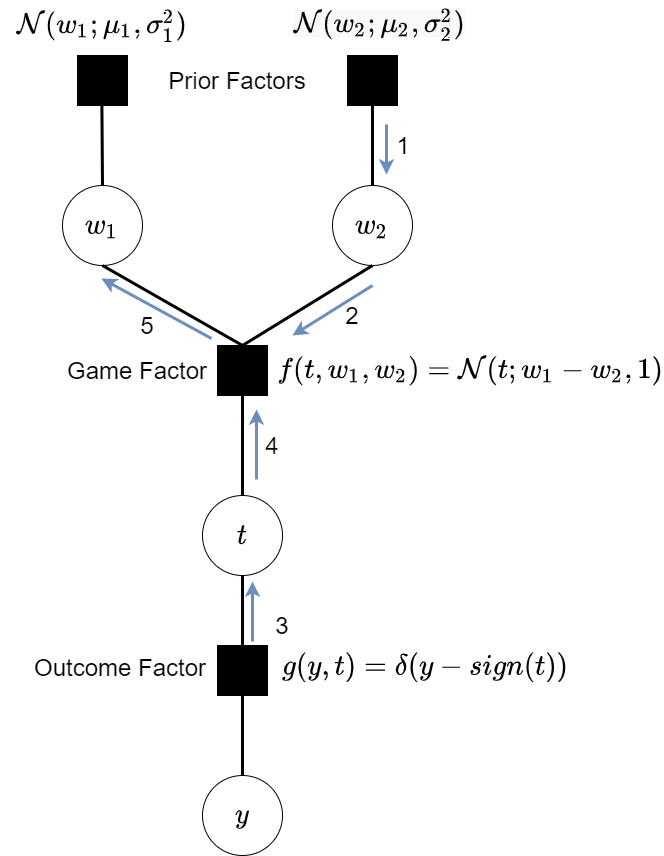
Let's now again use this model and the sum product message passing algorithm to compute the updated skill marginal for Player 1 in a game where Player 1 wins (a very similar sequence will give us the marginal for Player 2):
- First we pass messages from the prior factor attached to $w_2$ to the variable. This is simply: $$m_{prior \to w_2}=\mathcal{N}(w_2;\mu_2,\,\sigma_2^{2})$$
- Next we compute the message from the skill variables $w_2$ to the game factor $g$. There's only one other incoming message to $w_i$, the message that just arrived from the prior factor, so we simply pass that on. $$m_{w_2 \to f}=\mathcal{N}(w_2;\mu_2,\,\sigma_2^{2})$$
- We know that Player 1 won so we must have observed a the game outcome of $y=1$. Therefore we also pass a message from the outcome factor $g$ "up" to variable t. $$m_{g \to t} = \delta(1-sign(t))$$
- Again messages from variables to a factor are simply the product of all messages incoming to the variable except from that factor, so we simply pass the delta function along. $$m_{t \to f} = \delta(1-sign(t))$$
-
The message from the factor to $w_1$ is the product of the incoming messages from $t$ and $w_2$ and the
factor summing out all the variables except $w_1$.
$$m_{f \to w_1} = \Phi(\frac{\mu_2-w_1}{\sqrt{\sigma_2^{2}+1}})$$
\begin{align} m_{f \to w_1} &= \iint \! \delta(1-sign(t))\mathcal{N}(t;w_1-w_2,1)\mathcal{N}(w_2;\mu_2,\,\sigma_2^{2}) \, \mathrm{d}t\mathrm{d}w_2 \\ &= \int \! \delta(1-sign(t)) \int \mathcal{N}(t;w_1-w_2,1)\mathcal{N}(w_2;\mu_2,\sigma_2^{2}) \, \mathrm{d}w_2\mathrm{d}t \\ &= \int \! \delta(1-sign(t))\mathcal{N}(t;w_1-\mu_2,\sigma_2^{2}+1) \, \mathrm{d}t \\ &= \int_{0}^{\infty} \! \mathcal{N}(t;w_1-\mu_2,\sigma_2^{2}+1) \, \mathrm{d}t \\ &= \Phi(\frac{\mu_2-w_1}{\sqrt{\sigma_2^{2}+1}}) \end{align} Going from the second to third line I've used the result for the marginal distribution where the conditional and other marginal distribution are Gaussian. The proof and result can be found in Chapter 2.3.3 of [4].
- Finally we can work out the marginal distribution for $w_1$ by taking the product of all incoming factors. \begin{align} p(w_1) &= m_{f \to w_1} \times m_{prior \to w_1} \\ &= \mathcal{N}(w_1;\mu_1,\sigma_1^{2})\Phi(\frac{\mu_2-w_1}{\sqrt{\sigma_2^{2}+1}}) \end{align}
Another problem with our posterior..
A similar expression falls out for the updated skill marginal for $w_2$ by passing messages the other way. So we've got an expression for the posterior distributions for the skill variables having observed a game outcome, awesome. There's still a problem with this posterior though. We'd like to be able to use this posterior as the prior for the next game in which Player 1 plays. The problem that arises then is that because we have that pesky cumulative Gaussian left over upon playing the next game our new posterior will be the product of this prior with another cumulative Gaussian, taking us up to two cumulative Gaussians, a third game and we'll be at three cumulative Gaussians and so on till the $n^{th}$ game where we'll have accumulated $n$ cumulative Gaussian factors.
Each of these cumulative Gaussian factors has 2 parameters associated to it (as well as the original 2 parameters for the first Gaussian) and so after n games we will have $n*2+2=n+2$ parameters associated with a player's prior distribution. In other words the number of parameters required to represent a player's skill is $O(n)$. So the question is: can we get that $O(n)$ down to $O(1)$ space for each player? Well you won't be surprised that the folks that wrote the paper came up with a solution and that's what we'll talk about in the next section.
Expectation Propagation
Gaussian is good.
The intuition for solving the problem we encountered above comes (I believe) from the insight that if all our messages were Gaussian then when we multiplied them together the product would also be another Gaussian. So let's go back to our factor graph for the toy model and try and figure out where the non-Gaussian messages arose from. After a brief scroll up and down the page we're back and we see that it's step 3 in the above message passing that introduces the non-Gaussian message. If we want everything to be Gaussian then it might make sense to approximate this message as a Gaussian.
Of course there's a Bayesian ML technique for that called Expectation Propogation (EP) which allows us to approximate one probability distribution $p(x)$ with another one $q(x)$ by minimising the KL divergence between them. Further it turns out that if $q(x)$ is Gaussian then minimising the KL divergence is equivalent to moment matching whereby (for the 1d case) $p(x)$ has mean and variance equal to the mean and variance of $q(x)$.
There's still one issue though, unfortunately the distribution that we are trying to moment match (the delta function) doesn't have a well defined variance. That doesn't stop the authors of TrueSkill though, they use a little trick that is my favourite part of the paper to get round this problem.
A little trick
The trick then is rather than making an approximation to the message directly, we make a Gaussian approximation to the marginal distribution for the $t$ variable.
We already know what $m_{t \to f}$ is so let's quickly derive the "downwards" message.
$$m_{f \to t} = \mathcal{N}(t;\mu_1-\mu_2,1+\sigma_1^{2}+\sigma_2^{2})$$Now let's make our approximation to the marginal..
\begin{align} p(t) &= m_{f \to t} \times m_{t \to f} \\ &= \mathcal{N}(t;\mu_1-\mu_2,1+\sigma_1^{2}+\sigma_2^{2})\delta(1-sign(t)) \\ &\approx \mathcal{N}(t;\mu_{approx},\sigma_{approx}^{2}) \end{align} \begin{align} m_{t \to f} &= \frac{p(t)}{m_{f \to t}} \\ m_{t \to f} &= \frac{\mathcal{N}(t;\mu_{approx},\sigma_{approx}^{2})}{\mathcal{N}(t;\mu_1-\mu_2,1+\sigma_1^{2}+\sigma_2^{2})} \\ m_{t \to f} &= \mathcal{N}(t;\mu_{msg},\sigma_{msg}^{2}) \end{align} I've left out the nitty gritty details here for the sake of brevity. Going from the second to the third line is where we make our EP approximation and going from the penultimate to the final line we use the result that dividing two Gaussians gives you another Gaussian. If you would like to follow the the derivation in finer detail I go through that in the appendix. The point is that we've now got a Gaussian message going from variable $t$ to factor $f$!Finally our (approximate) Gaussian posterior!
We now have a Gaussian message passed "up" from the variable $t$ to the factor $f$. Let's now revisit our factor graph and complete the posterior calculation.
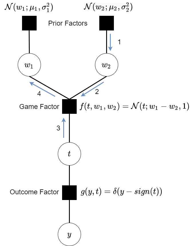
Let's now again use this model and the sum product message passing algorithm to compute the updated skill marginal for Player 1 in a game where Player 1 wins:
- Again we pass messages from the prior factors to the variable $w_2$. This is simply: $$m_{prior \to w_2}=\mathcal{N}(w_2;\mu_2,\,\sigma_2^{2})$$
- Same as before pass on the message through the variable as there are no other incoming factors. $$m_{w_2 \to f}=\mathcal{N}(w_2;\mu_2,\,\sigma_2^{2})$$
- We can now make use of our approximation for the message from $t$ to factor $f$. $$m_{t \to f} = \mathcal{N}(t;\mu_{msg},\sigma_{msg}^{2})$$
- We can now again pass a message from factor $f$ to the variable $w_1$. \begin{align} m_{f \to w_1} &= \iint \! \mathcal{N}(t;w_1-w_2,1)\mathcal{N}(t;\mu_{msg},\sigma_{msg}^{2})\mathcal{N}(w_2;\mu_2,\sigma_2^{2}) \, \mathrm{d}t\mathrm{d}w_2 \\ &= \mathcal{N}(w_1;\mu_{msg}+\mu_2,1+\sigma_{msg}^{2}+\sigma_2^{2}) \end{align} Again for the sake of not putting too much detail here I'll leave this derivation to the Appendix, but the most important insight is we still have a Gaussian message.
- Finally we can work out the marginal for $w_1$ by multiplying the message from the prior factor and from the game factor. \begin{align} p(w_1) &= m_{f \to w_1} \times m_{prior \to w_1} \\ &= \mathcal{N}(w_1;\mu_{msg}+\mu_2,1+\sigma_{msg}^{2}+\sigma_2^{2}) \mathcal{N}(w_1;\mu_1,\sigma_1) \\ &= \mathcal{N}(w_1;\mu_{new},\sigma_{new}) \end{align} Going from the second line to the final line we've used the result that multiplying two Gaussians also gives a Gaussian! So we've finally got our posterior and it's Gaussian!
What's the big deal...
That was a lot of effort to get a Gaussian posterior. The nice thing about having a Gaussian is that the posterior is now conjugate to the prior and so we can easily use this posterior as the new prior without having to worry about the form of the new posterior getting more complicated as we had before.
Conclusions
This has been a very brief summary of some parts of the TrueSkill paper. The paper describes a more general implementation of the toy model we've been dealing with that extends to teams of players, multiple teams playing against each other and handles draws to name a few of the details I've missed out here! I hope however that this has given you a broad intuition for the details that will allow you to better understand those. Anyway now that we have a better idea of what a player's skill is let's try and reanswer that to answer some of those questions we asked at the very start.
Who to rationally bet on in a game
For example if two players with skills $w_1$ and $w_2$ play each other what is the probability that each one wins. That's simply the likelihood we calculated earlier: $$p(y|w_1,w_2) = \Phi(y(w_1-w_2))$$
How can I rank players
We can also use these skills to rank players. I believe what's done in the TrueSkill implementation is a point estimate is taken from the marginal distribution for a players skill as $\mu-3\sigma$ as then there is a 99.7% chance that the player's skill is greater than that value. Once we have these point estimates they can then be used to rank the players in a leaderboard.
Other cool applications
One of the really fascinating implications of this modelling approach to estimating skills is that two players don't actually have to play each other for us to be able to rank them against each other. Players are simply ranked according to their performance against other players. A cool application of this was done by the Microsoft Research team who used TrueSkill to rank chess players across history [5], even though some were not even playing in the same time period!
Next steps
One of the things that the TrueSkill algorithm doesn't model is the score difference between players. For example if Player A beat me 10-0 in a game I would expect their skill update to be greater than if they struggled out a win at 10-9. This is something that I will be investigating and hopefully be able to talk about in a following blog post. Another thing I want to do is to use my Python implementation of TrueSkill to rank teams in the 2010 men's football world cup to try and predict the game outcomes in the knockout stages. I especially want to see if I can outpredict Paul the octopus because if I can't then really what's the point in learning all these Bayesian techniques, when I should just spend more time learning about octopi.
References
[1] Ralf Herbrich, Tom Minka, and Thore Graepel. TrueskillTM: a bayesian skill rating system. In Advances in neural information processing systems, pages 569–576, 2007.[2] Professor Carl Edward Rasmussen. Lecture notes. Probabilistic machine learning, 4F13. October 2019. University of Cambridge. [Online] Available from: http://mlg.eng.cam.ac.uk/teaching/4f13/1920/
[3] Moser J. The Math Behind TrueSkill. 2011. [Online] Available from: https://www.moserware.com/assets/computing-your-skill/The%20Math%20Behind%20TrueSkill.pdf [Accessed 14 June 2020].
[4] Bishop, Christopher M. Pattern Recognition and Machine Learning, 4 th edition. New York: Springer, 2006.
[5] P. Dangauthier, R. Herbrich, T. Minka, and T. Graepel. Trueskill through time: Revisiting the history of chess. In Advances in Neural Information Processing Systems 20, pages 337–344, 2008.